AutoScout

End-to-end AI system for automated American football film analysis.

1. What is AutoScout

AutoScout is an end-to-end AI system that automates American football film analysis by converting raw game footage into structured 2D player trajectories and tactical insights, reducing the need for manual expert annotation.

2. Motivation

Traditional football film study relies on labor-intensive manual analysis by domain experts, making it slow, costly, and difficult to scale, while existing computer-vision approaches typically address only isolated tasks such as formation recognition or field registration.

Motivated by the lack of a complete pipeline that handles multi-player detection under occlusion, spatial field mapping, and play-level interpretation, this project aims to deliver a unified system for scalable, objective football scouting.

3. Methodology

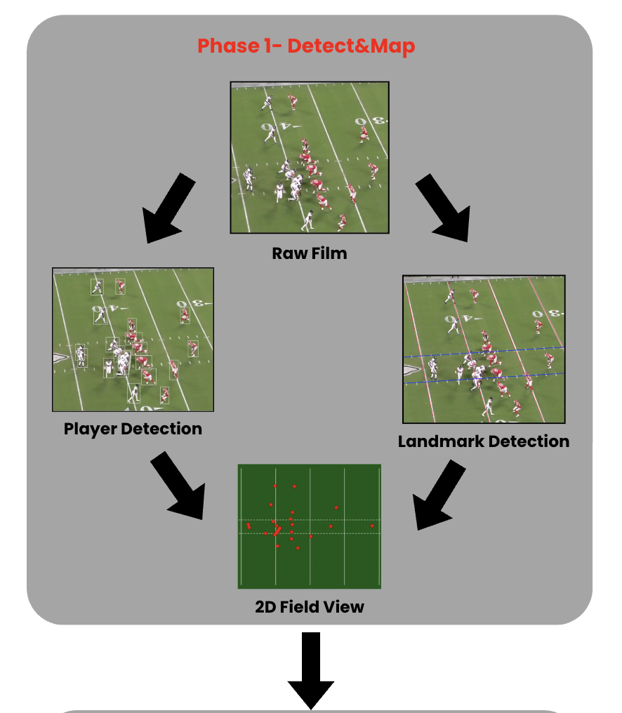
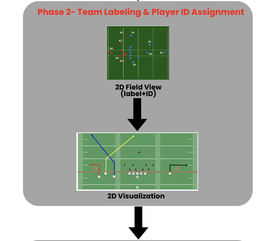
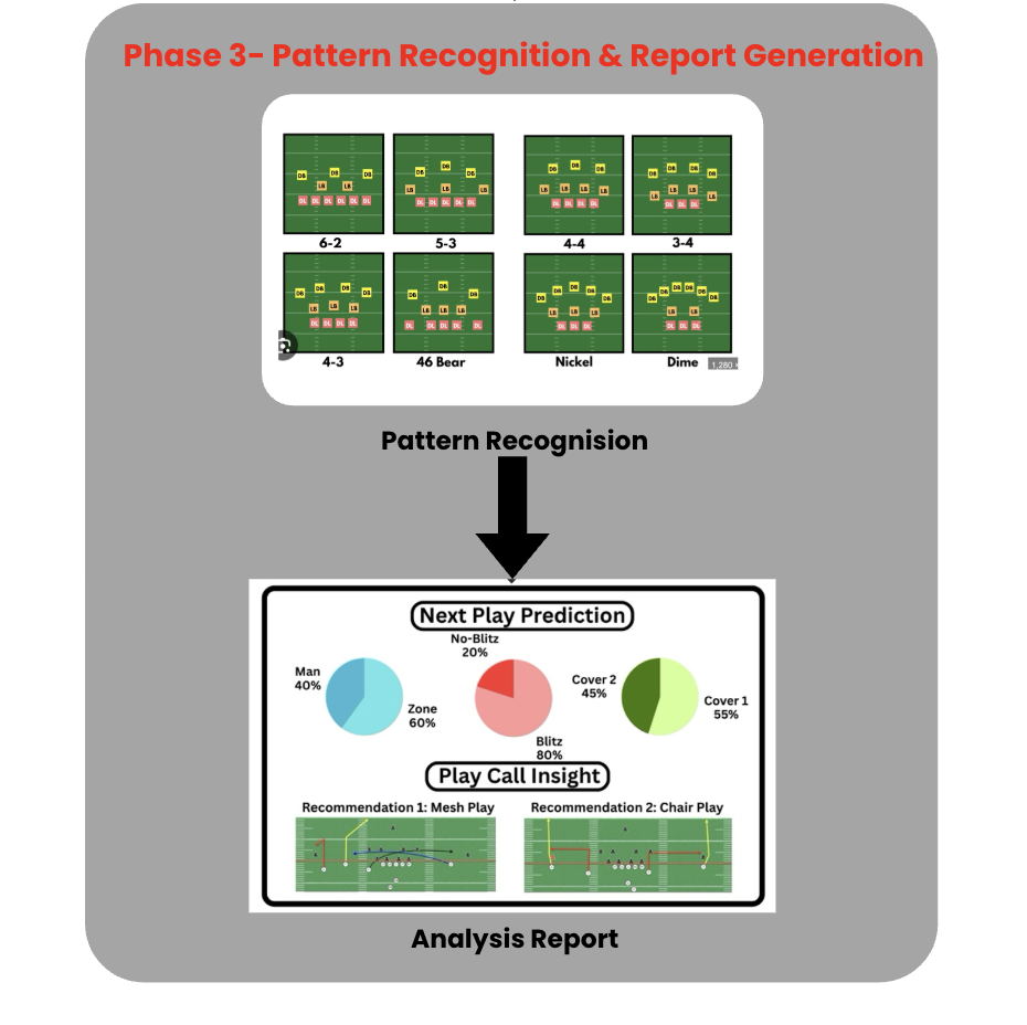
AutoScout consists of sequential phases that convert raw football footage into tactical insights. Phase 1 detects and maps player positions onto a 2D field, Phase 2 performs team labeling and persistent player ID assignment, and Phase 3 conducts pattern recognition and generates insight-driven analytical reports.

Figure 1: AutoScout workflow overview (Phase 1–3).

3.1 Phase 1 — Detect & Map

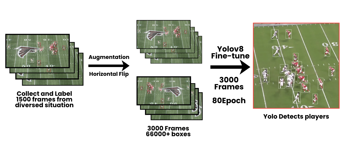
We manually annotated 1,500 broadcast frames, applied horizontal flip augmentation to expand the dataset to 3,000 frames with over 66,000 bounding boxes, and fine-tuned a YOLOv8 model for 80 epochs to detect all 22 on-field players, outputting their bounding boxes and image-space coordinates per frame.

Figure 2: YOLOv8 player detection training pipeline. — Figure 2. YOLOv8 player detection training pipeline.

We trained two YOLOv8 segmentation models—one for yard lines and one for hash marks—each using 700 annotated broadcast frames.

The intersections of the detected landmarks are paired with their known real-world field coordinates to compute a RANSAC-based homography for mapping broadcast-view positions to a canonical field.

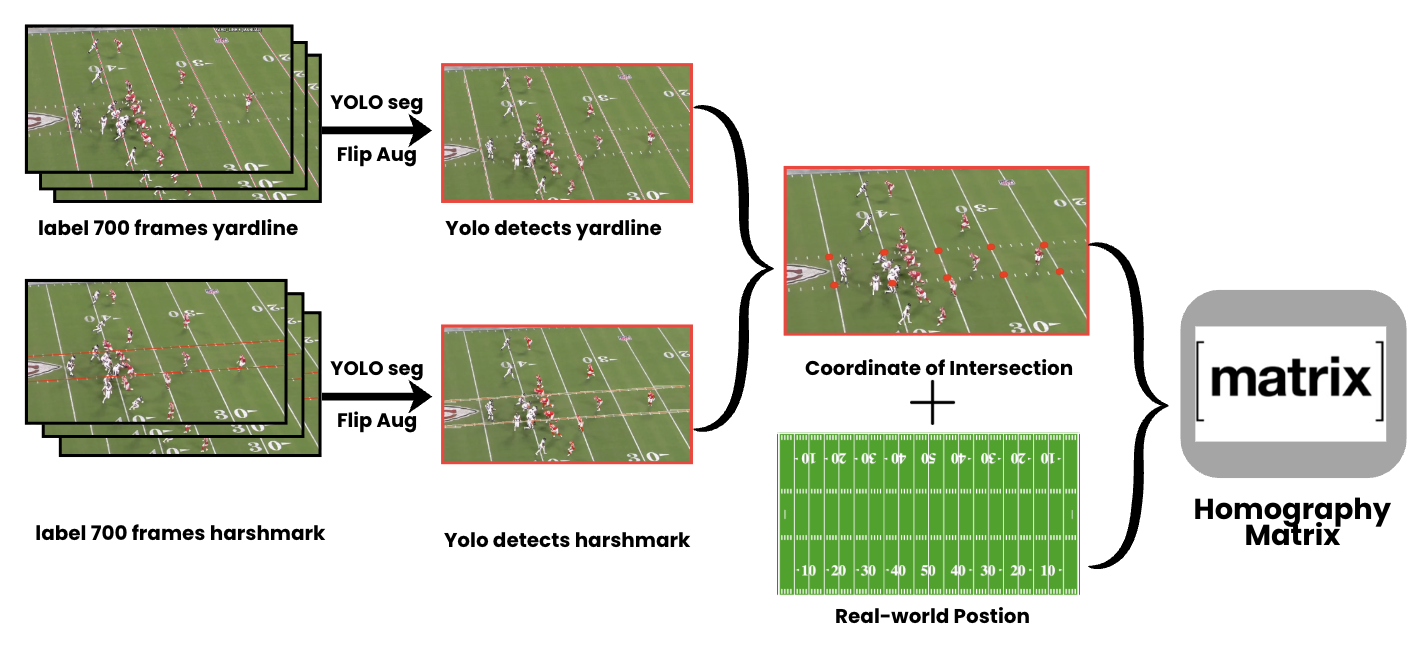
Figure 3: Landmark detection and homography estimation pipeline. — Figure 3. Landmark detection and homography estimation pipeline.

Using the estimated homography, broadcast-view player coordinates are projected into a canonical top-down field view for each frame, producing field-coordinate trajectories for downstream tracking and analysis.

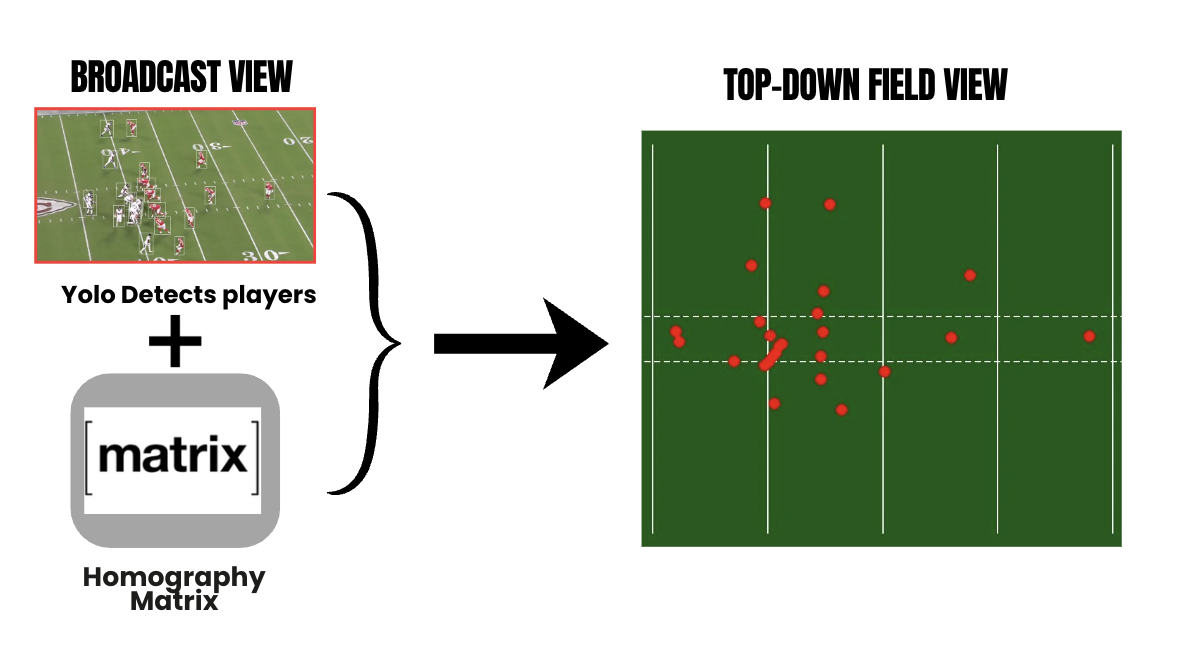
Figure 4: Projection from broadcast view to canonical top-down field view. — Figure 4. Projection from broadcast view to canonical top-down field view.

3.2 Phase 2 — Team Labelling & Player ID Tracking

For each detected player bounding box, we crop the jersey region and convert it from RGB to CIELAB color space.

We then extract per-channel mean and standard deviationfeatures and apply 2-means clustering to assign team labels corresponding to the two opposing teams.

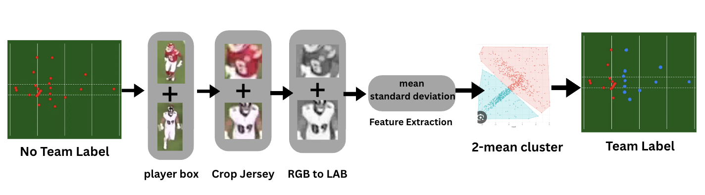
Figure 5: Team labeling via jersey color clustering. — Figure 5. Team labeling via jersey color clustering.

We use a Kalman filter–based tracking pipeline to predict each player’s position in the top-down field coordinate space across frames.

New detections are associated with predicted positions using nearest-neighbor matching based on Euclidean distance to maintain consistent player identities.

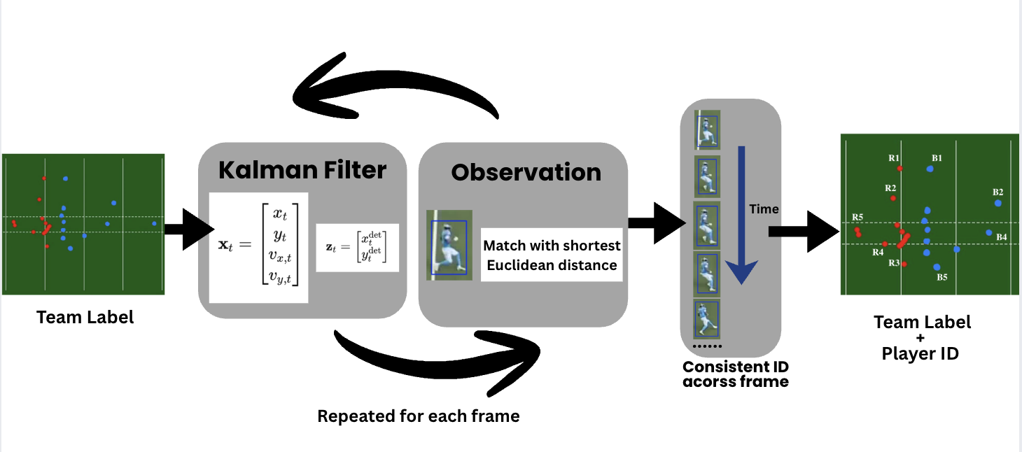
Figure 6: Kalman-filter tracking and data association for persistent player IDs. — Figure 6. Kalman-filter tracking and data association for persistent player IDs.

By combining team labeling and temporal tracking, Phase 2 produces a structured spatiotemporal representation where each player is assigned a team label and a persistent ID, enabling reliable 2D trajectory reconstruction and downstream tactical analysis.

3.3 Phase 3 — Pattern Recognition & Report Generation

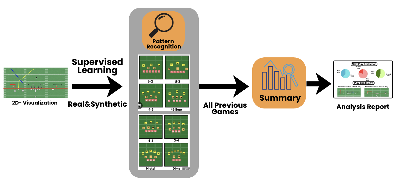
Using structured player trajectories from Phase 2, we train a supervised pattern recognition model on both real broadcast-derived data and manually constructed synthetic plays to identify formations, play types, and individual player behaviors.

The recognized patterns are aggregated across games to generate automated scouting reports summarizing opponent tendencies, play-calling distributions, and player-specific behaviors.

Figure 7: Pattern recognition and analysis report generation. — Figure 7. Pattern recognition and analysis report generation.

4. Model performance

4.1 Players Detection performance

As shown in Table 1, the YOLOv8 player detector achieves strong overall performance (mAP@0.5 = 0.98429, mAP@0.5:0.95 = 0.69246) with high precision (0.97442) and recall (0.95785). These results suggest the detector can reliably localize on-field players in broadcast frames, providing a stable input for subsequent projection and tracking stages.

Table 1: YOLOv8 player detection performance. — Table 1: Performance metrics of the YOLOv8 player detection model.

4.2 Yardline Detection performance

Table 2 shows that the yard-line model achieves excellent bounding-box detection performance (Box mAP@0.5 = 0.99489 and Box mAP@0.5:0.95 = 0.95219, with precision/recall near 0.99), indicating highly reliable localization of yard-line regions. In contrast, segmentation-mask metrics are notably lower (Mask mAP@0.5 = 0.75799; Mask mAP@0.5:0.95 = 0.26632). This gap is expected because yard lines form extremely thin structures in the image—often only a few pixels wide—so even minor boundary shifts during inference can cause a large drop in IoU, particularly under stricter IoU thresholds. Importantly, small pixel-level shifts in landmark detection do not significantly affect the resulting intersection point correspondences, and therefore have negligible impact on homography estimation and subsequent pipeline.

Table 2: Yard-line model performance. — Table 2: Performance metrics of the YOLOv8 yard-line model.

4.3 Hashmark Detection performance

Table 3 shows a performance trend similar to the yard-line model in Section 4.2, with strong bounding-box detection and lower segmentation-mask metrics due to the thin structure of hash marks. As with yard lines, these segmentation errors have minimal impact on landmark intersection extraction and downstream homography estimation.

Table 3: Hash mark model performance. — Table 3: Performance metrics of the YOLOv8 hash-mark model.